Introduction to Machine Learning in R

Authors: Raul Samayoa (@ralle123)
Lesson topic: Machine learning
Lesson content URL: https://github.com/UofTCoders/studyGroup/tree/gh-pages/lessons/r/ml-intro

Slides are available at this link

Demo examples:

Linear regression

#install.packages("lattice")
library(lattice)
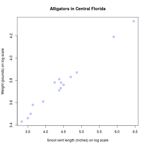
alligator <- data.frame(
  lnLength = c(3.87, 3.61, 4.33, 3.43, 3.81, 3.83, 3.46, 3.76,
    3.50, 3.58, 4.19, 3.78, 3.71, 3.73, 3.78),
  lnWeight = c(4.87, 3.93, 6.46, 3.33, 4.38, 4.70, 3.50, 4.50,
    3.58, 3.64, 5.90, 4.43, 4.38, 4.42, 4.25)
  )

# Plot our information
plot(
    alligator$lnWeight,
    alligator$lnLength,
    col = "blue",
    xlab = "Snout vent length (inches) on log scale",
    ylab = "Weight (pounds) on log scale",
    main = "Alligators in Central Florida"
    )

center

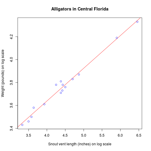
lm function fits a linear model. A typical model has the form response ~ terms

myModel <- lm(lnLength ~ lnWeight, data = alligator)

Visualize the regression

# Plot the chart with lm.
plot(
    alligator$lnWeight,
    alligator$lnLength,
    col = "blue",
    abline(myModel, col = 'red'),
    xlab = "Snout vent length (inches) on log scale",
    ylab = "Weight (pounds) on log scale",
    main = "Alligators in Central Florida"
    )

center

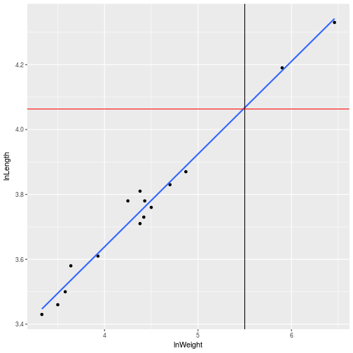
# Find weight of a alligator with weight of 5.5.
find_value <- data.frame(lnWeight = 5.5)
result <- predict(myModel, find_value)
result

##        1 
## 4.067312

If we trace the line with the value we are looking for we can see that the value seems correct

library(ggplot2)
end <- ggplot(alligator, aes(x = lnWeight, y = lnLength)) + 
    geom_point()
end + geom_smooth(method = 'lm', se = FALSE) + 
    geom_vline(xintercept = 5.5) + 
    geom_hline(yintercept = 4.06312, color = 'red')

center

k-means

library(datasets)
head(iris)

##   Sepal.Length Sepal.Width Petal.Length Petal.Width Species
## 1          5.1         3.5          1.4         0.2  setosa
## 2          4.9         3.0          1.4         0.2  setosa
## 3          4.7         3.2          1.3         0.2  setosa
## 4          4.6         3.1          1.5         0.2  setosa
## 5          5.0         3.6          1.4         0.2  setosa
## 6          5.4         3.9          1.7         0.4  setosa

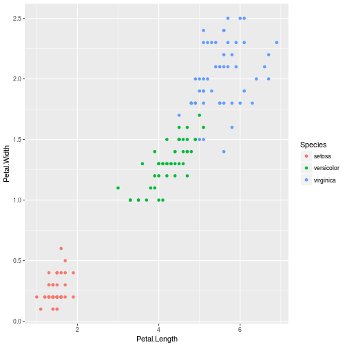
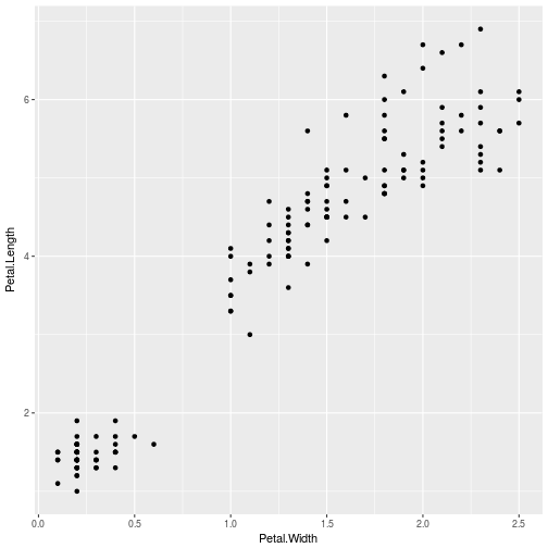
ggplot(iris, aes(Petal.Width, Petal.Length)) + 
    geom_point()

center

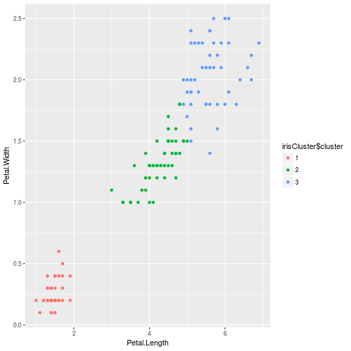
After resetting the seed I do a kmeans just selecting the 3-4 columns of iris, collect 3 iterations, selecting 20 random sets

set.seed(20)
irisCluster <- kmeans(iris[, 3:4], 3, nstart = 20)
#Comparing cluster with species
table(irisCluster$cluster, iris$Species)

##    
##     setosa versicolor virginica
##   1     50          0         0
##   2      0         48         4
##   3      0          2        46

We can graph our result

irisCluster$cluster <- as.factor(irisCluster$cluster)
ggplot(iris, aes(Petal.Length, Petal.Width, color = irisCluster$cluster)) + 
    geom_point()

center

Why did we do 3 clusters and not 4? dataset only has 3 species

ggplot(iris, aes(Petal.Length, Petal.Width, color = Species)) + 
    geom_point()

center