Cartography and Mapping in Python

Authors: Elliott Sales de Andrade
Research field: Seismology
Lesson topic: cartography, maps, projections, Python
Lesson content URL: https://github.com/UofTCoders/studyGroup/tree/gh-pages/lessons/python/cartography

# Default imports
import numpy as np
%matplotlib nbagg
import matplotlib.pyplot as plt

Setup

We will be using Cartopy for this lesson, so let’s import that. The common convention is to import it as follows:

import cartopy.crs as ccrs

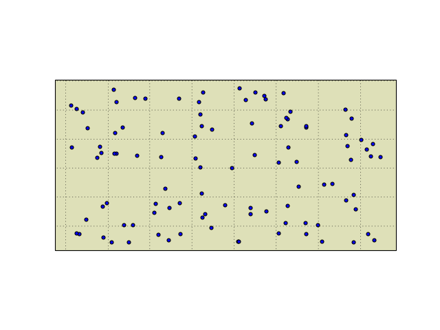
Let’s start with a simple plot of points:

np.random.seed(1)
x = 360 * np.random.rand(100)
y = 180 * np.random.rand(100) - 90

fig = plt.figure()
ax = fig.add_subplot(1, 1, 1)
ax.scatter(x, y)

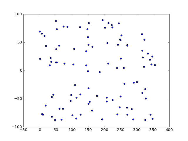
Why pick $x$ values between 0 and 360, and $y$ values between -90 and 90? Because that corresponds to the ranges for longitudes and latitudes! Let’s rename them.

lon = x
lat = y

Projections

The first problem with mapping is deciding in what projection to create the map. Some interesting properties you may want in a map are:

Conformal: Preserves angles locally, implying that locally shapes are not distorted.
Equal Area: Areas are conserved.
Compromise: Neither conformal nor equal-area, but a balance intended to reduce overall distortion.
Equidistant: All distances from one (or two) points are correct. Other equidistant properties are mentioned in the notes.
Gnomonic: All great circles are straight lines.

See the Wikipedia list of projections for more information.

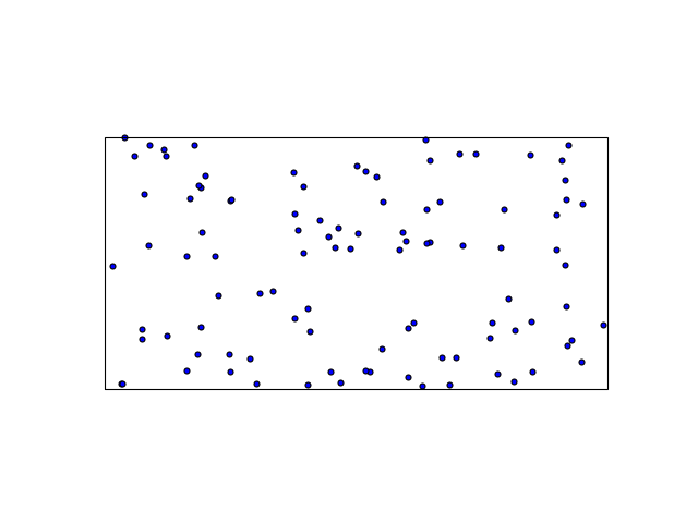
Cartopy has several options available. We will start with the very straightforward Plate Carrée (also known as Equirectangular or Equidistant Cylindrical.) We pass an instance of the projection class to the projection keyword argument of Figure.add_subplot to signify the projection in which the resulting map will be made.

fig = plt.figure()
ax = fig.add_subplot(1, 1, 1,
                     projection=ccrs.PlateCarree())
ax.scatter(lon, lat)

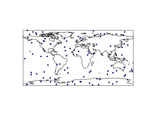
Adding elements

So far so good; let’s add some coast lines:

fig = plt.figure()
ax = fig.add_subplot(1, 1, 1,
                     projection=ccrs.PlateCarree())
ax.scatter(lon, lat)
ax.coastlines()

Or how about a land/ocean image:

fig = plt.figure()
ax = fig.add_subplot(1, 1, 1,
                     projection=ccrs.PlateCarree())
ax.scatter(lon, lat)
ax.stock_img()
ax.coastlines()

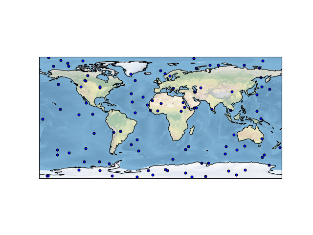
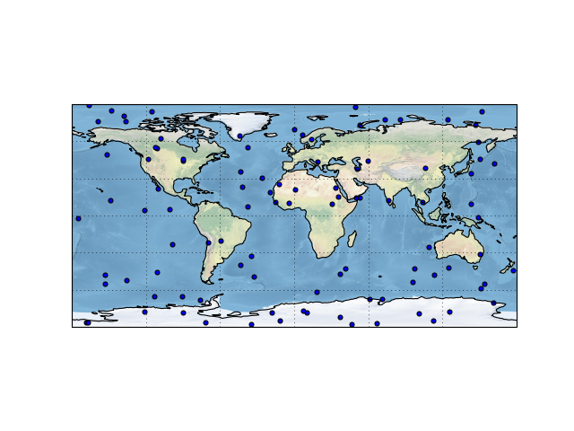
And maybe some grid lines:

fig = plt.figure()
ax = fig.add_subplot(1, 1, 1,
                     projection=ccrs.PlateCarree())
ax.scatter(lon, lat)
ax.stock_img()
ax.coastlines()
ax.gridlines()

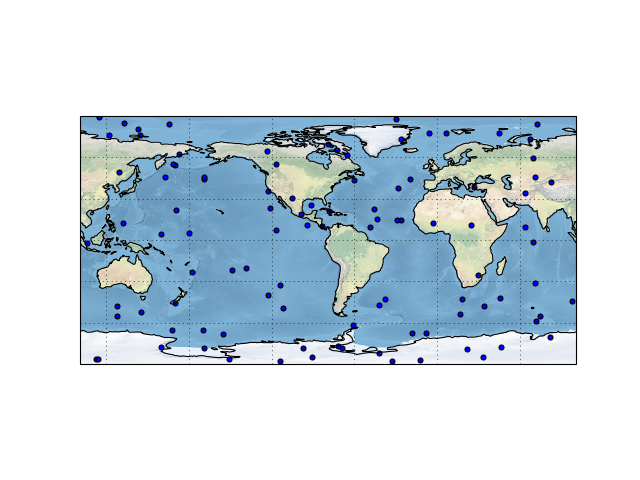
This projection supports two arguments:

ccrs.PlateCarree?

fig = plt.figure()
ax = fig.add_subplot(1, 1, 1,
                     projection=ccrs.PlateCarree(central_longitude=-79))
ax.scatter(lon, lat)
ax.stock_img()
ax.coastlines()
ax.gridlines()

Other projections

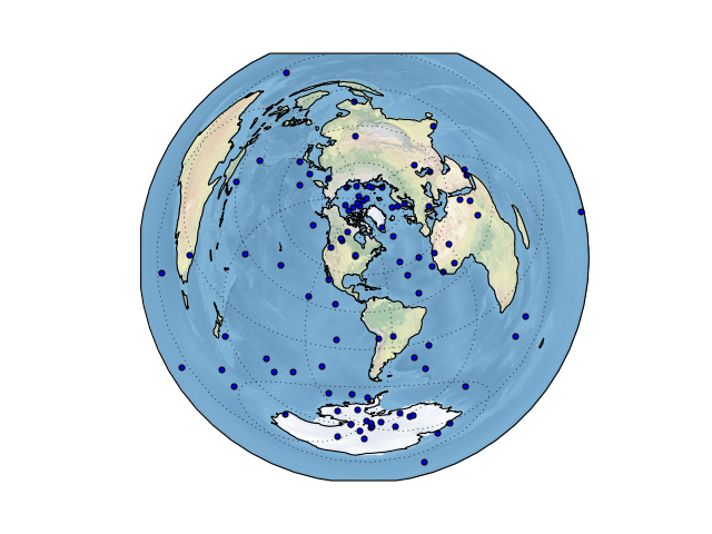
Let’s try out a different projection now, say Azimuthal Equidistant. It preserves angles and distances from the centre of the map. We’ll centre it on this building, 43.660924°N, 79.398329°W.

to_lon = -79.398329  # East is positive.
to_lat = 43.660924

fig = plt.figure()
ax = fig.add_subplot(1, 1, 1,
                     projection=ccrs.AzimuthalEquidistant(central_longitude=to_lon,
                                                          central_latitude=to_lat))
ax.scatter(lon, lat)
ax.stock_img()
ax.coastlines()
ax.gridlines()

Hmm, what happened? Our points should be all over the globe. Actually, if you look at the previous plot, even though we changed the central longitude, the points never moved either!

This is a common trap with Cartopy, but it’s also one of its most useful features. We neglected to specify the projection in which the scatter points originated, thus it was plotted in the map coordinates. Map coordinates are almost always specified in metres (except for Plate Carrée) and since our points are in degrees, they are extremely small (the circumference is approximately 40,000 km.)

We can specify the input projection using the transform= keyword argument to ax.scatter. In this case, we use the Geodetic projection for the points. This projection is basically longitude/latitude.

fig = plt.figure()
ax = fig.add_subplot(1, 1, 1,
                     projection=ccrs.AzimuthalEquidistant(central_longitude=to_lon,
                                                          central_latitude=to_lat))
# Here we add the transform argument and use the Geodetic projection.
ax.scatter(lon, lat, transform=ccrs.Geodetic())
ax.stock_img()
ax.coastlines()
ax.gridlines()

What’s the difference between Plate Carrée and Geodetic? Let’s look at a map:

ff_lon = 8 + 41 / 60
ff_lat = 50 + 7 / 60

fig = plt.figure()
ax = fig.add_subplot(1, 1, 1,
                     projection=ccrs.PlateCarree(central_longitude=(to_lon + ff_lon) / 2))
ax.plot([to_lon, ff_lon], [to_lat, ff_lat], c='b', lw=2,
        transform=ccrs.PlateCarree())
ax.plot([to_lon, ff_lon], [to_lat, ff_lat], c='r', lw=2,
        transform=ccrs.Geodetic())
ax.set_global()
ax.stock_img()
ax.coastlines()
ax.gridlines()

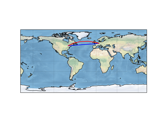
As you can see, Plate Carrée uses the straight-line path on a longitude/latitude basis, while Geodetic uses the shortest path in a spherical sense (the geodesic.)

Features

Let’s focus in on Canada for a bit to see what features Cartopy can depict. We’ll switch to the Lambert Conformal Conic projection which works well for this size and range of the map, and is recommended by StatsCan. We’ll use their recommended standard parallels (see wiki link for explanation) of 49°N and 77°N, and a central longitude of 91°52’W. The boundaries are arbitrarily chosen to be 63°W to 123°W and 37°N to 75°N, and set with ax.set_extent.

# An arbitrary choice.
canada_east = -63
canada_west = -123
canada_north = 75
canada_south = 37

standard_parallels = (49, 77)
central_longitude = -(91 + 52 / 60)

fig = plt.figure()
ax = fig.add_subplot(1, 1, 1,
                     projection=ccrs.LambertConformal(central_longitude=central_longitude,
                                                      standard_parallels=standard_parallels))
ax.set_extent([canada_west, canada_east, canada_south, canada_north])
ax.stock_img()
ax.coastlines()
ax.gridlines()

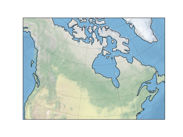
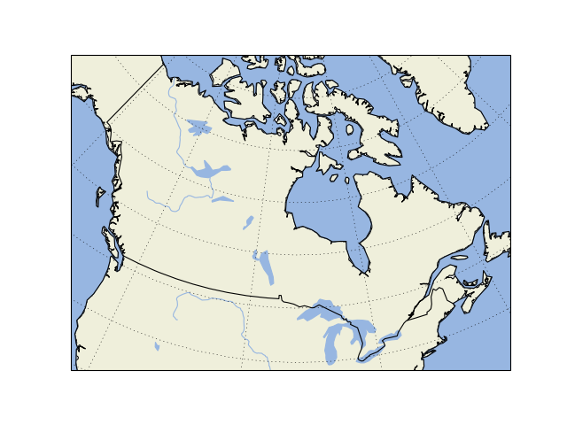
Here we can see two things:

The stock image and coastlines are not very high resolution.
The coastlines only show the oceanic coast; no lakes or rivers, and certainly no countries.

Cartopy provides various “features” that can provide some or all of this content at varying resolutions. Some simple shortcuts to Natural Earth data are provided in the cartopy.feature module and can be added via ax.add_feature. These are downloaded and cached on the fly, so there may be some issues if the WiFi is being flaky in MP408.

import cartopy.feature as cfeature

fig = plt.figure()
ax = fig.add_subplot(1, 1, 1,
                     projection=ccrs.LambertConformal(central_longitude=central_longitude,
                                                      standard_parallels=standard_parallels))
ax.set_extent([canada_west, canada_east, canada_south, canada_north])
ax.gridlines()
ax.add_feature(cfeature.OCEAN)
ax.add_feature(cfeature.LAND)
ax.add_feature(cfeature.LAKES)
ax.add_feature(cfeature.BORDERS)
ax.add_feature(cfeature.COASTLINE)
ax.add_feature(cfeature.RIVERS)

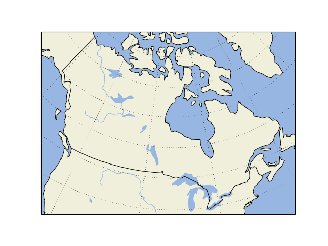
These are all defined on the 1:110m(illion) scale, but what if we want something a bit higher resolution? Well, the above were just shortcuts and we can use cfeature.NaturalEarthFeature directly with its scale argument.

land_50m = cfeature.NaturalEarthFeature('physical', 'land', '50m',
                                        edgecolor='k',
                                        facecolor=cfeature.COLORS['land'])

fig = plt.figure()
ax = fig.add_subplot(1, 1, 1,
                     projection=ccrs.LambertConformal(central_longitude=central_longitude,
                                                      standard_parallels=standard_parallels))
ax.set_extent([canada_west, canada_east, canada_south, canada_north])
ax.gridlines()
ax.add_feature(land_50m)
ax.add_feature(cfeature.LAKES)
ax.add_feature(cfeature.OCEAN)
ax.add_feature(cfeature.BORDERS)
ax.add_feature(cfeature.COASTLINE)
ax.add_feature(cfeature.RIVERS)

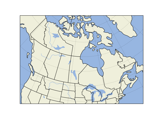
Now, let’s add the provinces and states (the possible names as used here can be determined by visiting the link above):

provinces_50m = cfeature.NaturalEarthFeature('cultural',
                                             'admin_1_states_provinces_lines',
                                             '50m',
                                             facecolor='none')

fig = plt.figure()
ax = fig.add_subplot(1, 1, 1,
                     projection=ccrs.LambertConformal(central_longitude=central_longitude,
                                                      standard_parallels=standard_parallels))
ax.set_extent([canada_west, canada_east, canada_south, canada_north])
ax.gridlines()
ax.add_feature(cfeature.LAND)
ax.add_feature(cfeature.LAKES)
ax.add_feature(cfeature.OCEAN)
ax.add_feature(cfeature.BORDERS)
ax.add_feature(cfeature.COASTLINE)
ax.add_feature(cfeature.RIVERS)
ax.add_feature(provinces_50m)

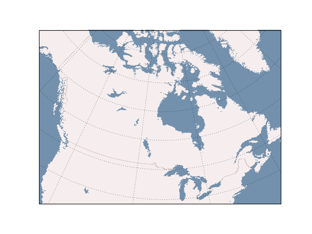
Web Services

Web Map Services (WMS) provide vector data as a download via some web API and Web Map Tile Services provide raster data via a similar interface.

These can be added by ax.add_wms and ax.add_wmts.

fig = plt.figure()
ax = fig.add_subplot(1, 1, 1,
                     projection=ccrs.LambertConformal(central_longitude=central_longitude,
                                                      standard_parallels=standard_parallels))
ax.set_extent([canada_west, canada_east, canada_south, canada_north])
ax.gridlines()

ax.add_wms(wms='http://vmap0.tiles.osgeo.org/wms/vmap0',
           layers=['basic'])

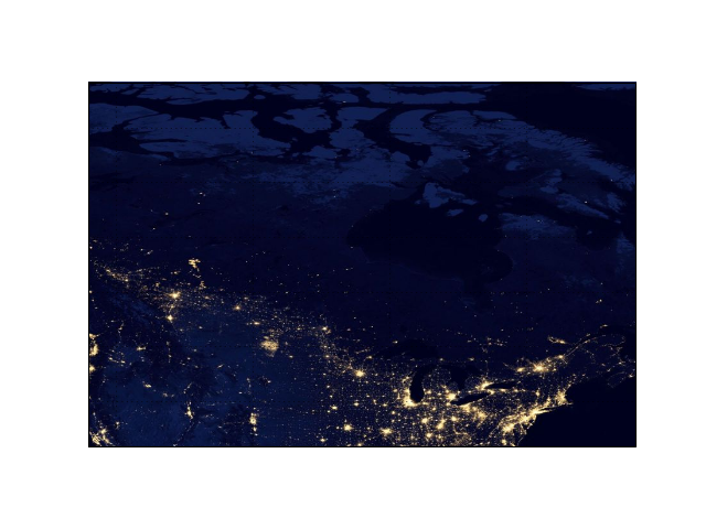
Unfortunately, WMTS doesn’t support reprojection in 0.14, but it will in the next release 0.15, so we need to use Plate Carrée for this map.

url = 'https://map1c.vis.earthdata.nasa.gov/wmts-geo/wmts.cgi'
layer = 'VIIRS_CityLights_2012'

fig = plt.figure()
ax = fig.add_subplot(1, 1, 1,
                     projection=ccrs.PlateCarree())
ax.set_extent([canada_west, canada_east, canada_south, canada_north])
ax.gridlines()
ax.add_wmts(url, layer)

Shapefile I/O

What about outlines that you provide yourself? You might obtain a shapefile from somewhere outlining something. These can be read with cartopy.io.shapereader.Reader.

from cartopy.io.shapereader import Reader

We will use the data files provided with the lesson here:

data = Reader('icitw_wgs84')

fig = plt.figure()
ax = fig.add_subplot(1, 1, 1,
                     projection=ccrs.LambertConformal(central_longitude=central_longitude,
                                                      standard_parallels=standard_parallels))
ax.set_extent([-79.6, -79.2, 43.5, 43.9])
ax.gridlines()

ax.add_geometries(data.geometries(), crs=ccrs.Geodetic(), edgecolor='k', facecolor='none')

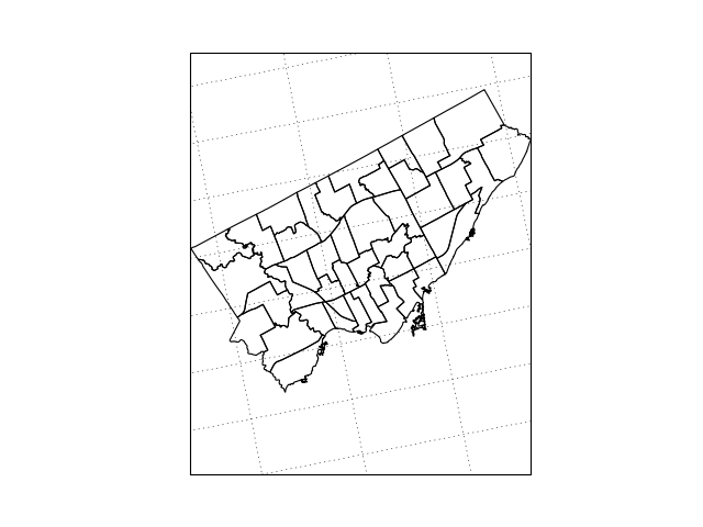
In case you do not recognize the shapes, these are wards for the city of Toronto.

Each of those geometries is a shapely object, on which we can do things like determine if points are contained. We won’t really go into any details of it here, though. The example below is just a quick one-off to show how it might be used.

import shapely.geometry as sgeom

ward = next(data.geometries())

us = sgeom.Point(to_lon, to_lat)
ward.contains(us)

False

fig = plt.figure()
ax = fig.add_subplot(1, 1, 1,
                     projection=ccrs.LambertConformal(central_longitude=central_longitude,
                                                      standard_parallels=standard_parallels))
ax.set_extent([-79.6, -79.2, 43.5, 43.9])
ax.gridlines()

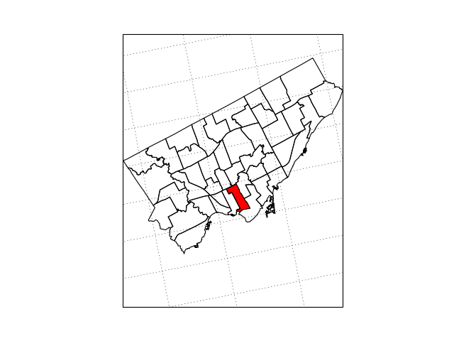
for ward in data.geometries():
    if ward.contains(us):
        our_ward = ward
        ax.add_geometries(our_ward, crs=ccrs.Geodetic(), edgecolor='k', facecolor='r')
    else:
        ax.add_geometries(ward, crs=ccrs.Geodetic(), edgecolor='k', facecolor='none')

What happened here? It turns out that the ward data is a bit buggy, and each ward is not a closed polygon.

our_ward.is_closed

False

Shapely will nicely render its contents in a notebook:

our_ward

svg

The type can be found from the geom_type property:

our_ward.geom_type

'MultiPolygon'

MultiPolygon contains multiple polygons, but fortunately, there’s just the one.

len(our_ward)

We’ll construct a “linear ring” (basically a closed shape) from the data in the first polygon.

sgeom.LinearRing(our_ward[0].exterior.coords)

svg

And if we use that in our plot, the fill colour will no longer “spill” out over the rest of the map.

fig = plt.figure()
ax = fig.add_subplot(1, 1, 1,
                     projection=ccrs.LambertConformal(central_longitude=central_longitude,
                                                      standard_parallels=standard_parallels))
ax.set_extent([-79.6, -79.2, 43.5, 43.9])
ax.gridlines()

for ward in data.geometries():
    if ward.contains(us):
        # Close the polygon...
        our_ward = [sgeom.LinearRing(ward.geoms[0].exterior.coords)]
        ax.add_geometries(our_ward, crs=ccrs.Geodetic(), edgecolor='k', facecolor='r')
    else:
        ax.add_geometries(ward, crs=ccrs.Geodetic(), edgecolor='k', facecolor='none')